The question is a bit confused in it's use of statistical terminology and ideas, but I think there is an answer, so I'll address the terminology as I go:
From a frequentist standpoint, each spin of a fair roulette wheel is
an independent event with a 50% chance of landing on black.
A Bayesian would also view it as an independent event. If events are independent, it just means the probability of one event does not depend on another event. As others have pointed out, saying that it is a "fair"" roulette wheel is essentially asserting that it has a probability of 50% of landing on black (I'm assuming there isn't a green zero slot). But that is what we are testing, so a frequentist would only assume it is fair to set up a "Null hypothesis".
According to this view, no matter how many consecutive black outcomes
are observed, the probability of the next spin being black remains 50%
Again, a Bayesian would take that view as well.
On the other hand, the Bayesian approach involves updating our beliefs
based on new evidence.
I think this is a misunderstanding of Bayesianism, taken in conjunction with the statement about frequentists in particular viewing the events as independent. In this scenario, a Bayesian would also model the events as independent, with a fixed, but unknown probability of landing on black. When we get data, the probability that the roulette wheel lands on black doesn't change (it is fixed by the physics of the wheel), what changes is our state of knowledge (a.k.a. belief) regarding the value of that probability.
Before getting to the methods:
Specifically, how do we balance the theoretical independence of events
with the practical improbability of long sequences of identical
outcomes in a fair game?
This is a misunderstanding, and can't be answered. Both Bayesians and frequentists would treat the events as independent, so there is nothing to balance. In both Bayesian and frquentist approaches there is a fixed probability of landing heads, but we don't know what it is.
There are various ways this problem can be approached, but the frequentist is limited by defining probabilities only in terms of a long run frequency. This means they can't assign a probability to the truth of a particular proposition, such as "the wheel is fair" or "the probability of landing black lies in some particular interval" - these are either true or false, and have no non-trivial long run frequency (i.e. other than zero or one). The Bayesian on the other hand, can assign a probability to a particular event the truth of a proposition, so they can give a more direct answer.
FREQUENTIST
What a frequentist would probably do is to use a Null Hypothesis Statistical Test (NHST). They would begin by setting out their null hypothesis (the hypothesis that must be nullified in order to claim that the wheel is rigged). In this case H0: p(black) = p(red) = 0.5. They would then evaluate the p-value, which is the probability of a sequence of events at least as extreme as that actually observed. To keep it simple, lets assume we observed the wheel landing on black five consecutive times. Under H0:
p = 0.5^5 = 0.03125
If this value was below the significance level, alpha, then the frequentist would say "the null hypothesis can be rejected" and then act as if the wheel was rigged.
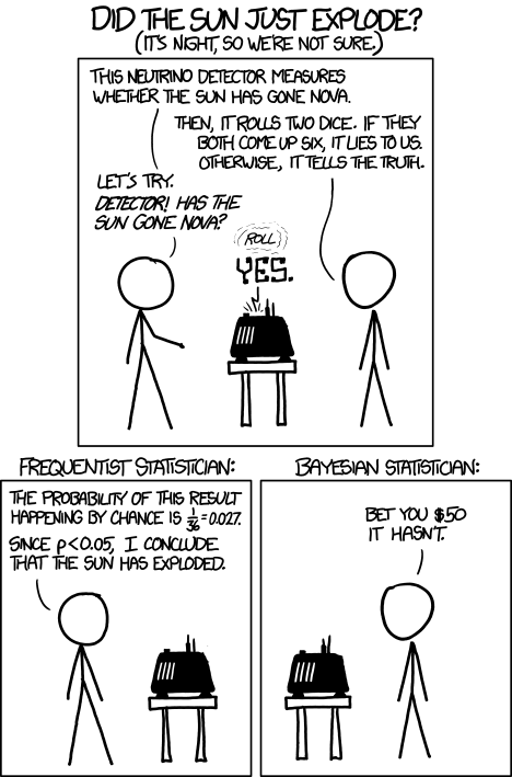
The tricky bit here is working out the appropriate "significance level". People often opt for 95% level (expressed as 1-alph), but Gigerenizer views this as "Mindless statistics" and part of the "Null ritual" because it is symptomatic of the common use of NHSTs without a solid understanding of the frequentist framework, which commonly leads to misunderstandings. This is well illustrated by the XKCD cartoon

The error the frequentist is making here is to use a significance level that is far too lax, and a much smaller value of alpha is appropriate. The probability that the sun has actually gone nova is vanishingly small, so it would be unreasonable to continue with that hypothesis because the alarm would have a 1-in-20 probability of going off if it was due to chance!
Another tricky issue here, when performing an NHST, we say "we can reject H0" or "we fail to reject H0". This rather clunky wording is highlighting the fact that rejecting H0 does not mean we "accept" H1 - in this case, it is not evidence that the sun has gone nova. The reason we can't say that is because the test does not involve the prior probabilities or the likelihood of the observation if it were caused by H1. NHSTs are best viewed as being like Popperian falsification. The best we can say about H1 is that it has survived an attempt at falsification, however the severity of the attempt may be pretty low (as in this case) and so the corroboration of H1 may be rather slim!
So how should we choose the significance level? Many frequentists are not going to like this, but the truth is that it is a subjective choice of the statistician, based on their prior knowledge of the system, often with no straightforward means of calculating what it should be. The inventor of significance testing, Sir Ronald Fisher, wrote:
… no scientific worker has a fixed level of significance at which from
year to year, and in all circumstances, he rejects hypotheses; he
rather gives his mind to each particular case in the light of his
evidence and his ideas.
The really awkward bit is that you can't make this choice by assigning probabilities to your prior beliefs and working out the significance level, because frequentists fundamentally cannot assign a probability to the truth of a proposition. This also means that there generally
isn't a straightforward means of calculating what the significance level should be for some particular purpose, and the statistician will generally opt for a value that "seems about right". Frequentism is often viewed as being objective, but this isn't true, it still contains subjective elements and prior beliefs, but they are often ignored and (often deeply inappropriate) default values used instead.
Now, that would be a reasonable answer if you just looked at one set of five spins of the wheel. If you waited for five consecutive spins that landed black, then wait long enough and it will happen, even if the wheel is fair. To get around that, you could introduce corrections for the implicit "multiple hypothesis testing" (i.e. you are performing many tests, not just one). It gets complicated, but the significance level remains arbitrary subjective choice, with no clear method of calculating it.
Another issue is that no real roulette table will be exactly fair. It will always have some asymmetry such that the probability of landing on black is not exactly 0.5. This means in practice, if you collect enough data, you will always be able to show that the wheel is rigged, even if it is the fairest wheel ever constructed. This is because the H0 is based on a point value from a continuous distribution, so the probability of observing a particular point value is zero. You could get around this by defining H0 using an interval centered on 0.5, but that makes calculating the p value more difficult and probably not worth it. If it takes 1,000,000 spins to detect the bias, common sense should tell you that it is of no practical significance, even if it is of "statistical significance".
@DoubleKnot raises a very good point in the comments. If we observe a sequence of spins that all land on black, then we can just monitor the p-value to see when it gets a low enough value that we should be suspicious of bias. However, another way to look at the question is to ask how many spins of the wheel do we have to observe in order to be confident that if the null hypothesis was false that we would confidently expect the test to have rejected it. This is a sample size calculation, and it can be based on an analysis of statistical power. The power of a test is the probability of rejecting the null hypothesis if it is actually false, and it is usually denoted as beta.
This is something that users of NHSTs rarely consider, which is part of the "Null Ritual" mentioned earlier. One of the tricky aspects in this case is that the power of the test depends on how rigged the wheel is. If it always lands on black, you should be able to reject H0 fairly quickly. If it is only rigged by a few percentage points (which would give a healthy profit for the casino in the long run) then you would need much more data. This makes the calculation more tricky. I have a blog post, "What does Statistically Significant Actually Mean?", at SkepticalScience, which contains a worked example for flipping a coin, which is a very similar problem.
BAYESIAN
The frequentist approach tends to be fairly easy to implement (which is perhaps why it is used more often), but as can be seen above, the underlying framework is very subtle and it can be quite easy to misinterpret the results (often by interpreting a probability as the probability of the truth of a proposition - e.g. the p-value falacy where the p-value is assumed to be the probability that H0 is true).
The Bayesian approach is generally the other way round - it is conceptually a lot more straightforward, and less prone to misinterpretation, but tends to be more difficult to perform as it often requires integral calculus, and we often need bespoke solutions for every problem. Some cases are reasonably easy to perform though.
A Bayesian can directly assign a probability to the truth of a proposition, e.g. the probability that the wheel is rigged. This is because for a Bayesian, a probability is a measure of (relative) plausibility, and is not necessarily defined to be a long run frequency. However, in this case, a better place to start is estimating how biased the wheel is, i.e. the probability of landing on black. Rather than have a single probability, a Bayesian would instead have a probability distribution representing their state of knowledge about the value of that probability (yes a probability of a probability). The reason for doing so is to correctly represent our uncertainty about the value of that probability.
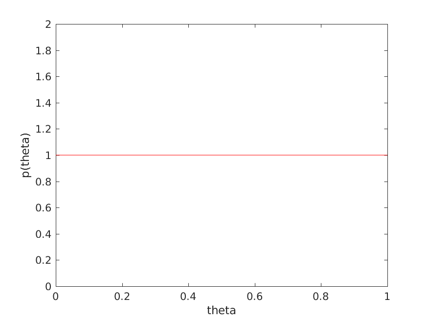
An objectivist Bayesian might start from a prior belief that represented complete ignorance of the value of the probability, which I will call theta, in this case a uniform prior on the interval [0, 1]. For technical reasons, we would do this using a Beta(1,1) distribution

As observations arrive, we then update this prior using Bayes rule,
P(theta|obs) = p(obs|theta)p(theta)/p(obs)
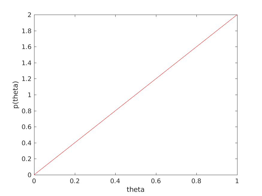
For a roulette wheel spin, which can land on black or red, the likelihood p(obs|theta) is a Bernoulli distribution (or Binomial for multiple spins). The reason for using a Beta prior is that it is the conjugate prior for Bernoulli and Binomial likelihoods, which means that the posterior obtained by Bayes rule will also be a Beta distribution. If you work out the maths (which I can't do here as there is no LaTeX support), if you observed the wheel landing on black, then the posterior belief would be a beta(2,1) distribution (note you have ruled out landing on black is impossible, theta = 0):

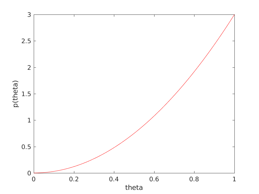
if you observe the wheel landing on black a second time, you get a Beta(3,1) posterior:

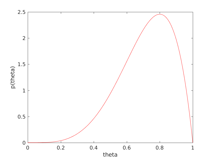
and so on. Say we observe the wheel landing on black twice more, and red once, we would have a Beta(5,2) posterior

Note I have done this from memory, without checking, so I may have got something wrong - caveat lector!
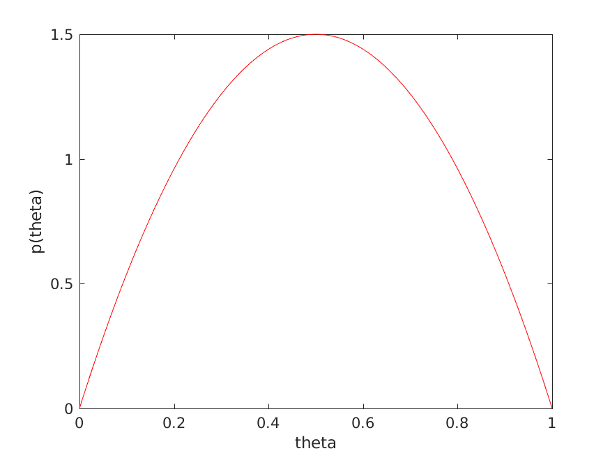
A subjectivist Bayesian would have started with a more informative prior, encoding that it would be difficult to make a very biased wheel (and that a casino owner would have to be very stupid to try!), and use a Beta distribution that was peaked around theta = 0.5, say a Beta(2,2) distribution (which is not very informative):

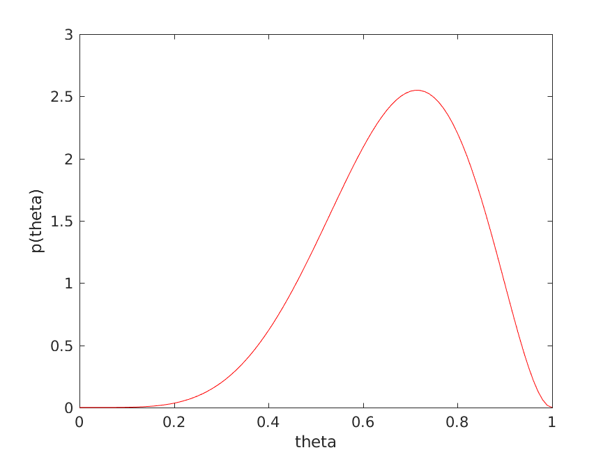
Some people dislike the subjectivity of informative prior, however this prior is more in accord with rational expectations (knowing how roulette wheels operate) than the uninformatve flat prior. If we have the same set of observations, and push them through Bayes' rule, we end up with a Beta(6,3) posterior:

Note that the peak of this posterior is closer to 0.5 because of the prior knowledge imposed by the prior, which is peaked at 0.5. Note that you can see that the prior is effectively adding some "virtual" observations, one black and one red for the Beta(1,1) and two black and two red for the Beta(2,2) prior.
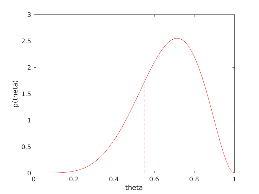
So, now to work out the probability that the table is rigged. Unfortunately the probability according to our posterior that the wheel is exactly fair, i.e. theta = 0.5, is zero. This is because theta is a continuous variable, so the probability of any specific value is zero. The solution is to define an interval around 0.5 that we would consider to be fair for practical purposes, say [0.45 - 0.55]. We can work out the probability of the table being fair by integrating our posterior over that interval

I worked this out numerically to be approximately p(fair) = 0.1317, implying that p(rigged) = 1 - p(fair) = 0.8683
Alternatively, you could use Bayes rule more directly, as in @causative's answer - but the difficulty there is that you need to know the degree to which the wheel is rigged to calculate p(obseration|rigged), or you could adopt a prior distribution for that as well and integrate it out of the calculation (marhginalisation). In this particular case, I think the approach I have given here is a bit easier to follow, but should give the same result.
Now this probability is the probability that the wheel is
fair/rigged, assuming the statistical model is right, so while there is still an issue of what the threshold should be, reasoning in terms of probabilities is a lot more natural than reasoning with "significance" or "confidence" levels (which sound like statements about plausibility, but unfortunately aren't).
What I would do is adopt a minimum risk strategy, and work out the cost of accusing the casino of using a rigged wheel when it is actually fair, and the cost of playing at the casino assuming that the wheel is fair when it is actually rigged. I can then work out how much I would expect to loose by choosing to denounce the casino or not, which is based on the costs and the probabilities I have already calculated. So for Bayesian probability there is a rational consistent approach, which is know as Bayesian decision theory.
CONCLUSION
Frequentism is conceptually tricky and easy to misinterpret, but easy to implement. Unfortunately the threshold where we decide to denounce the casino is difficult to define and depends on prior probabilities, which frequentists often discourage us from using because they are viewed as subjective.
Bayesianism on the other hand is conceptually easier, but you often need to end up doing integral calculus, which is enough to put a lot of people off using them. Defining the threshold is easier because we can directly express the probability that the wheel is rigged, which a frequentist can't.
However, this doesn't mean that one framework is right and the other is wrong - both are useful and it is a good idea to have both sets of tools in your toolbox and know how to use them (and how not to misuse them).

